Brief Introduction to R & Feature Transformation
Chris Hodapp hodapp87@gmail.com
CincyFP, 2016 December 13
Front matter
This is all done in Jupyter (formerly IPython) and IRkernel.
Visit http://159.203.72.130:8888 to use this same notebook in your browser.
(...unless you're reading this later, of course. Go fire up your own docker container with "docker run -d -p 8888:8888 jupyter/r-notebook" or something.)

(thanks Creighton)
What is R?
- An interpreted, dynamically-typed language based on S and made mainly for interactive use in statistics and visualization
- Sort of like MATLAB, except statistics-flavored and open source
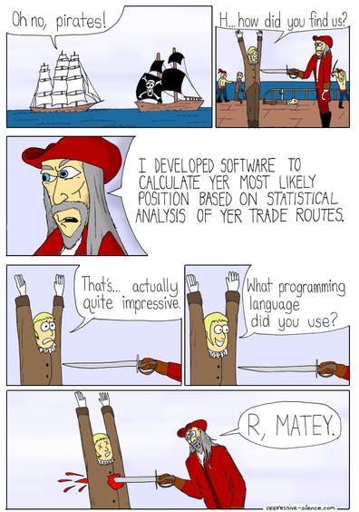
- A train-wreck that is sometimes confused with a real programming language.
- "R is a dynamic language for statistical computing that combines lazy functional features and object-oriented programming. This rather unlikely linguistic cocktail would probably never have been prepared by computer scientists, yet the language has become surprisingly popular." (Evaluating the Design of the R Language)
- The R Inferno (Patrick Burns), http://www.burns-stat.com/pages/Tutor/R_inferno.pdf
So... why use it at all?
- Stable and documented extensively!
- Excellent for exploratory use interactively!
- Epic visualization!
- Magical, fast, and elegant for arrays, tables, vectors, and linear algebra!
- Huge standard library!
- Packages for everything else on CRAN!
- Still sort of FP!
- Excellent tooling! (Sweave, Emacs & ESS mode, RStudio, Jupyter...)
How do I use R?
Do you need plotting or visualization? Use ggplot2. Completely ignore built-in plotting.
Do you need something else? Search CRAN.
Does no CRAN package solve your problems? Do you need to write "real"(tm) software for production? Strongly consider giving up.
Obligatory R notebook demonstration...
Dataframes
- A sort of blending of matrices, arrays, and database tables. Type is per-column.
- Accessed by row range, column range, or both.
Many imitators:
- Python: Pandas, http://pandas.pydata.org/
- Stricter indexing (oriented for time-series)
- Scala, Java, Python: Apache Spark DataFrame
- Tied to Spark SQL & Catalyst; weakly-typed distributed
Dataset
- Tied to Spark SQL & Catalyst; weakly-typed distributed
- Haskell: Frames, https://github.com/acowley/Frames
- Clojure: Incanter (?), http://incanter.org/
- Julia: https://github.com/JuliaStats/DataFrames.jl
dplyr
- See: Introduction to dplyr, https://cran.rstudio.com/web/packages/dplyr/vignettes/introduction.html
filter,slice- Select rows (filter is by predicate, slice is by position)arrange- Reorder rowsselect,rename- Select columnsdistinct- Choose only distinct rowsmutate,transmute- Make new columns from existing onessummarise- 'Peel off' one grouping level (or collapse frame to one row) with aggregate functionssample_n,sample_frac- Randomly sample (by count or by percentage)group_by- Group observations (most of above worked on grouped observations)- All dplyr calls are side-effect-free, and
x %>% f(y) = f(x,y) - Bonus: This all works on remote SQL databases too (and
data.tableviadtplyr)
Motivating Example
- Example data set from: https://archive.ics.uci.edu/ml/datasets/Letter+Recognition
- 20,000 samples, 16 dimensions
Unsupervised Learning
- Sometimes a precursor to supervised learning
- Sometimes done for its own sake
- Some broad (and overlapping) categories:
- Latent variable models
- Clustering
Curse of Dimensionality (Bellman)


- Intuition from k-nearest neighbor: If each sample occupies a certain amount of 'space' in the input space, the number of samples required to still 'cover' that space increases exponentially with the number of dimensions. (That's the hand-waving description. See Vapnik-Chervonenkis dimension and Computational Learning Theory.)
- If possible: Don't add more dimensions. Either reduce dimensions, or increase samples.
- But... how to remove dimensions?
Feature Transformation
General form
$$x : \mathcal{F}^N \mapsto \mathcal{F}^M, M < N$$(though actually M >> N is useful too and is the basis for kernel methods such as SVMs)
Subsets
- Feature Selection: Loosely, throw away dimensions/features.
- Information gain, Gini index, entropy, variance, statistical independence...
- Filtering: Reduce features first, and then perform learning. Learning can't feed information 'back' to filtering.
- Wrapping: Reduce features based on how learning performs.
- Forward search: Add features one by one. At each step, add the feature that helps the learner the most.
- Backward search: Remove features one by one. At each step, discard the feature that impacts the learner the least.
- e.g. 4-dimensional feature space mapped to 2 dimensions, $(x_1, x_2, x_3, x_4) \mapsto (2x_1-x_2, x_3 + x_4)$
Then for $X$ containing samples as row vectors, $Y=X\mathcal{P}_x$: $$ \mathcal{P}_x= \begin{bmatrix} 2 & 0 \\ -1 & 0 \\ 0 & 1 \\ 0 & 1 \end{bmatrix} $$
Consider data expressed as an $n\times m$ matrix with each column representing one feature (of $m$) and each row one sample (of $n$):
$$ X= \begin{bmatrix} a_1 & b_1 & c_1 & \cdots\\ a_2 & b_2 & c_2 & \cdots\\ a_3 & b_3 & c_3 & \cdots\\ \vdots & \vdots & \vdots & \ddots\\ a_n & b_n & c_n & \cdots\\ \end{bmatrix} $$- Focus on first feature $A=\left\{a_1, a_2, \dots\right\}$
- Mean = $\left\langle a_i \right\rangle_i = \frac{1}{n} \sum_i^n a_i=\mu_A$
- $\left\langle \dots \right\rangle$ = expectation operator
- Variance: $$\sigma_A^2=\left\langle \left(a_i-\left\langle a_j \right\rangle _j\right)^2 \right\rangle_i=\left\langle \left(a_i-\mu_A\right)^2 \right\rangle_i = \frac{1}{n-1}\sum_i^n \left(a_i-\mu_A\right)^2$$
(if you want to know why it is $\frac{1}{n-1}$ and not $\frac{1}{n}$, ask a statistics PhD or something)
- Consider another feature $B=\left\{b_1, b_2, \dots\right\}$, and assume that $\mu_A=\mu_B=0$ for sanity
- Covariance of $A$ and $B$: $$\sigma_{AB}^2=\left\langle a_i b_i \right\rangle_i=\frac{1}{n-1}\sum_i^n a_i b_i$$
- If $\sigma_A^2=\sigma_B^2=1$ then $\sigma_{AB}^2=\rho_{A,B}$ (correlation)
Treating $A$ and $B$ as vectors:
$$\sigma_{AB}^2=\frac{A\cdot B}{n-1}$$Recalling our data matrix:
$$ X= \begin{bmatrix} a_1 & b_1 & c_1 & \cdots\\ a_2 & b_2 & c_2 & \cdots\\ a_3 & b_3 & c_3 & \cdots\\ \vdots & \vdots & \vdots & \ddots\\ a_n & b_n & c_n & \cdots\\ \end{bmatrix} $$It can be rewritten as column vectors:
$$ X= \begin{bmatrix} a_1 & b_1 & c_1 & \cdots\\ a_2 & b_2 & c_2 & \cdots\\ a_3 & b_3 & c_3 & \cdots\\ \vdots & \vdots & \vdots & \ddots\\ a_n & b_n & c_n & \cdots\\ \end{bmatrix} =\begin{bmatrix} A & B & C & \cdots \end{bmatrix} $$Then covariance matrix is:
$$\mathbf{S}_X=\frac{X^\top X}{n-1}= \begin{bmatrix} \sigma_{A}^2 & \sigma_{AB}^2 & \sigma_{AC}^2 & \sigma_{AD}^2 & \cdots \\ \sigma_{AB}^2 & \sigma_{B}^2 & \sigma_{BC}^2 & \sigma_{BD}^2 & \cdots \\ \sigma_{AC}^2 & \sigma_{BC}^2 & \sigma_{C}^2 & \sigma_{CD}^2 & \cdots \\ \sigma_{AD}^2 & \sigma_{BD}^2 & \sigma_{CD}^2 & \sigma_{D}^2 & \cdots \\ \vdots & \vdots & \vdots & \vdots & \ddots \end{bmatrix} $$- Square ($m \times m$), symmetric, variances on diagonals, covariances off diagonals
- If all features are completely independent of each other, all covariances are 0.
- That is: Covariance matrix is a diagonal matrix (all zeros, except for diagonal).
- So... What is this matrix $P$ such that for $Y=XP$, covariance matrix $\mathbf{S}_Y$ is diagonal?
- Like basically every other question in linear algebra, the answers are:
- Eigendecomposition
- SVD
- That magical transform matrix $P$ equals a matrix whose columns are eigenvectors of $X^\top X$. (Left as an exercise for the reader.) Since covariance matrix $X^\top X$ is a symmetric and positive semidefinite matrix, its eigenvectors form an orthogonal basis with non-negative eigenvalues (obviously).
- Eigenvectors are the principal components of $X$.
- Corresponding eigenvalues are the variance of $X$ 'along' each component (also equal to the diagonals of $\mathbf{S}_Y$) - or the 'variance explained' by each component.
Dimensionality Reduction
- $P$ is an $m\times m$ matrix. Every column is a component, and assume they are in descending order of variance (almost all eigendecomposition implementations do this regardless).
- Data matrix $X$ is $n \times m$.
- $Y=XP$ then is also $n \times m$, and is the result of projecting each sample in $X$ onto each component.
- In effect, a coordinate transform
- A reversible one; since $P$ is an orthogonal basis, $P^{-1}=P^\top$, $X=YP^\top$
- $Y$ is in a new space, still $m$-dimensional.
- 1st column = 1st dimension = $X$'s projection on most important component
- 2nd column = 2nd dimension = $X$'s projection on 2nd most important component
- and so on.
- Two equivalent ways of reducing dimensionality:
- Throw away "less important" dimensions from the end of $Y$, e.g. let $Y_d$ = the 1st $d$ columns of $Y$ ($n\times d$ matrix)
- Or, let $P_d$ equal the first $d$ columns of $P$ ($m\times d$ matrix), then $Y_d=XP_d$
- Rule of thumb: Keep enough dimensions for 90% of total variance
- 'Lossy' reconstruction back into original $m$-dimensional space: $\hat{X}=Y_dP_d^\top$
Principal Component Analysis
- We have thus just derived (in abbreviated fashion) a ridiculously useful tool called PCA (Principle Component Analysis).
- It's often done with SVD rather than eigendecomposition (better-behaved numerically, provides other information)
- It is a linear algebra method that tries to find uncorrelated Gaussians. Uncorrelated sometimes coincides with statistically independent.
- The almost-completely-unrelated ICA (Independent Component Analysis) derives independent features using probability and information theory.
Random Projections / RCA
- This is a stupid, stupid algorithm that shouldn't work:
- Pick $m$ random directions in the $n$-dimensional space, $m < n$.
- Project the $n$-dimensional data onto them.
- Is the projection good enough (e.g. low reprojection error)?
- Yes: You're done.
- No: Repeat step 1.
- It does work - very quickly, and irritatingly well.
References Used
- Official R intro: https://cran.r-project.org/doc/manuals/R-intro.html
- Evaluating the Design of the R Language (Morandat, Hill, Osvald, Vitek): http://r.cs.purdue.edu/pub/ecoop12.pdf
- PCA Tutorial: http://www.cs.princeton.edu/picasso/mats/PCA-Tutorial-Intuition_jp.pdf
- Machine Learning (Mitchell)
- Ch. 11, Mining of Massive Datasets (Leskovec, Rajaraman, Ullman): http://infolab.stanford.edu/~ullman/mmds/book.pdf
Other Links
- Impatient R, http://www.burns-stat.com/documents/tutorials/impatient-r/
- R: The Good Parts, http://blog.datascienceretreat.com/post/69789735503/r-the-good-parts
- Two excellent textbooks, freely available as PDFs:
- ISLR (Intro. to Statistical Learning in R): http://www-bcf.usc.edu/~gareth/ISL/
- ESL (Elements of Statistical Learning): http://statweb.stanford.edu/~tibs/ElemStatLearn/